KO: One-Dimensional Hydrocode (KO)
Introduction
Steps to get started with KO (see details below)
1. Obtain terminal (Mac-OSX) or CygWin (PC) access and install gfortran
2. Download, compile and run the KO hydrocode example
3. Install either Matlab or Octave (free open-source version of Matlab) for post processing
4. Load KO output into Matlab or Octave and plot using jmovie_ko.m script
1. Obtain terminal and install GFortran (If you have a terminal you can skip)
PC Users
- If you have a PC, you can install CygWin and gfortran on your PC by watching this video. If you already have a terminal emulator and a copy of gfortran you can skip to step 2, as there is nothing special about the install outlined in the video.
Mac/Linux Users
- If you have a Mac/Linux, terminal is an app that comes with OSX. You can open from Applications/Utilities.
- If you don't have a copy of gfortran, you can use Homebrew to install by watching this video
2. Download, compile and run the KO hydrocode example
a. Download KO which is located at the bottom of this webpage.
b. Place the downloaded files in a directory on your computer.
c. Open Cygwin/Terminal and goto the directory where you put the KO files. In Cygwin/Terminal you have to use the change directory command (ie cd 'c:\...') that is described in the video. You can type 'ls' d. to see a listing of the files in the directory and 'pwd' will tell you what directory you are in.
e. Compile the KOv13.f by typing 'gfortran KOv13.f' into Cygwin/Terminal; this will create an executable named 'a.exe' in the KO directory.
f. Run this executable by typing './a.exe' on a PC or './a.out' on a Mac/Linux
g. If the code runs to completion, you see "** Finished!! ***" and have a ko.dat file in your KO directory
3. Install Matlab or GNU-Octave for post processing
Matlab:
Matlab is a powerful numeric matrix/data manipulations and plotting code. It requires a license. Your home institution may provide a license to you. If you don't have a license you can install the OpenSource version of Matlab which is called Octave.
Octave for PC or Mac/Linux:
You can download a free copy of GNU-Octave by clicking the download button in upper-right and following the directions. Alternatively for the Mac/Linux install it is easy to download the latest dmg file from github . I am running 6.2.0
4. Load KO output into Matlab/Octave and run jmovie_ko post-processing script
a. Open matlab/octave and change the local directory to the KO directory
b. Load the ko.dat data into matlab/octave by typing 'load ko.dat'
c. After it loads you can plot the data by typing 'jmovie_ko'
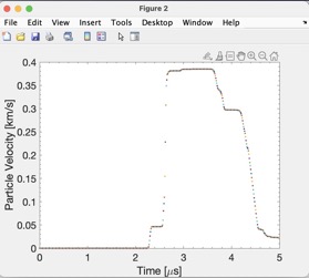
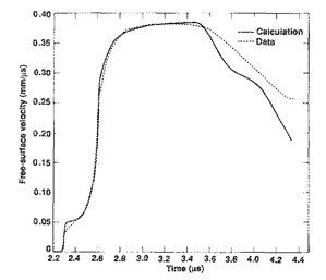
d. Your plot should look like the plot shown below. Notice how it compares to the data from the Steinburg paper also shown below.
e. At this point you are ready for the workshop! If you want to learn more and watch some instructional videos about KO you can go here.
- KO output
- Figure 6 from Steinberg-JAP-1989
KO Hydrocode
 The following hydrocode is based on a book by Mark Wilkins entitled "Computer Simulation of Dynamic Phenomena". The code is a simple one-dimensional Lagrangian finite difference hydro-dynamic scheme, with von Mises strength. I have included several user selectable equations of state including ideal gas, Mie-Gruenisen and p-alpha. The code is written in fortran and the data can be visualized in matlab or octave, which is an open source free version of matlab. I have also made a couple of quick you-tube videos that show you how to compile, run and visualize the results.
Download: Click on the following link to download the source code (KOv13.f), input file (ko.in) and post-processing file input file (jmovie_ko.m). You might also find the appendices and the property tables from Wilkins book helpful.
KO: Quick Start
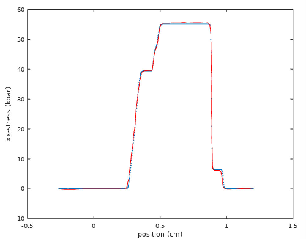
The following video shows you how to download and compile KO using gfortran. It introduces a simple example of an aluminum flyer impacting a stationary aluminum target at 700 m/s. This video also introduces the post-processing visualization within Octave, which is the open-source version of Matlab. Everything described herein will also work in Matlab. The last part of the video demonstrate how to visualize a movie generated from the Al-Al impact within octave. You can download the entire directory I use in this video from (Example-Fig3-8.zip) which also contains the discretized data from Figure 3.8 from Wilkins book.See video in YouTube
KO: Shock Hugoniot Example Problem
 |
|---|
| Output from example problem of aluminum impacting aluminum at 700 m/s |
See video in YouTube
KO: Post-processing using Octave/Matlab and jmovie_ko.m
This video presents a short tutorial on how data within ko.dat is formatted and written to file. It then presents a short tutorial on how to use the m-file jmovie_ko.m to plot data contained in ko.dat as either a movie or an xy plot.See video in YouTube
KO: Input File
This video presents more detail regarding the KO input file (ko.in) and its format. It reviews the equations of state and boundary conditions implemented in KO and how to select and implement them for a simulation. The video connects the fortran files, and sections of the code, to the stencil in Wilkins' book.See video in YouTube
KO: Explained
The following video goes into painful detail regarding how the KO hydrocode is constructed in Fortran following the derivation in Mark Wilkins book. There is some discussion of how the code is structured and hidden features, as well as how data is stored. If you have any additional questions about KO, I would be happy to discuss.See video in YouTube
Please e-mail john.borg at MU.edu with any questions you might have regarding this code.